Introduction to delimtools • delimtools

Rationale

There are at least three major steps when doing single-locus species delimitation analysis:

Preparing your data;
Running species delimitation analysis;
Visualizing results.

The rationale of delimtools is to provide helper functions for all these steps. This guide introduces you to these functions and shows how to apply them to your datasets. In this tutorial, we will use the geophagus dataset provided in this package. This dataset contains 354 cytochrome c oxidase sequences of the Geophagus sensu stricto species group downloaded from GenBank. Most of these sequences are from the data analysed by Ximenes et al. (2021) and is documented in ?geophagus.

Preparing your data

Usually, our main source of information for single-locus species delimitation analysis is a FASTA formated file containing nucleotide sequences. The most straighforward way to import a FASTA formated file to R Environment is by using ape::read.FASTA():

path_to_file <- system.file("extdata/geophagus.fasta", package = "delimtools")

geophagus <- ape::read.FASTA(file= path_to_file)

Since geophagus dataset is provided along with delimtools, one can simply call it directly:

geophagus
#> 354 DNA sequences in binary format stored in a list.
#> 
#> All sequences of same length: 690 
#> 
#> Labels:
#> MZ504301.1
#> MZ504328.1
#> MZ504318.1
#> MZ504313.1
#> MZ504311.1
#> MZ504312.1
#> ...
#> 
#> Base composition:
#>     a     c     g     t 
#> 0.237 0.282 0.178 0.303 
#> (Total: 244.26 kb)

Check identifiers across files

Although the header of each sequence in a FASTA file may contain information about the source organism from which the sequence was obtained, we recommend storing this information in a tabular format file (e.g. csv, tsv, xlsx, etc.), using an unique sequence identifier for both FASTA and tabular files. We can have a glimpse of our sequence metadata by checking geophagus_info:

dplyr::glimpse(geophagus_info)
#> Rows: 354
#> Columns: 19
#> $ scientificName        <chr> "Geophagus_altifrons", "Geophagus_altifrons", "G…
#> $ scientificNameGenBank <chr> "Geophagus altifrons", "Geophagus altifrons", "G…
#> $ class                 <chr> "Teleostei", "Teleostei", "Teleostei", "Teleoste…
#> $ order                 <chr> "Cichliformes", "Cichliformes", "Cichliformes", …
#> $ family                <chr> "Cichlidae", "Cichlidae", "Cichlidae", "Cichlida…
#> $ genus                 <chr> "Geophagus", "Geophagus", "Geophagus", "Geophagu…
#> $ dbid                  <dbl> 2063684375, 2063684465, 2063684523, 2063684453, …
#> $ gbAccession           <chr> "MZ504486.1", "MZ504531.1", "MZ504560.1", "MZ504…
#> $ gene                  <chr> "coi", "coi", "coi", "coi", "coi", "coi", "coi",…
#> $ length                <dbl> 659, 699, 627, 612, 552, 654, 627, 651, 666, 609…
#> $ organelle             <chr> "mitochondrion", "mitochondrion", "mitochondrion…
#> $ catalogNumber         <chr> "1614", "17578", "1616", "1194", "2748", "1610",…
#> $ country               <chr> "Brazil: Tapajós- Jacareacanga- Pará", "Brazil: …
#> $ publishedAs           <chr> "Mapping the hidden diversity of the Geophagus s…
#> $ publishedIn           <chr> "Unpublished", "Unpublished", "Unpublished", "Un…
#> $ publishedBy           <chr> "Ximenes,A.M.", "Ximenes,A.M.", "Ximenes,A.M.", …
#> $ date                  <chr> "25-OCT-2021", "25-OCT-2021", "25-OCT-2021", "25…
#> $ decimalLatitude       <dbl> -6.276008, -3.449100, -6.276008, -1.501489, -6.1…
#> $ decimalLongitude      <dbl> -57.74000, -57.73533, -57.74000, -52.68211, -48.…

It’s desirable that both our FASTA file and our metadata have the same dimensions and no abscent, mistyped, or duplicated sequence identifiers within and between these files. Let’s check if our FASTA file and our metadata has the same sequence identifiers using delimtools::check_identifiers():

check_identifiers(data= geophagus_info, identifier= "gbAccession", dna= geophagus)
#> ✔ Identifiers are the same across files.

Now, let’s omit the first 10 sequences and check again:

check_identifiers(geophagus_info, "gbAccession", geophagus[11:354])
#> Error in `check_identifiers()`:
#> ! Identifiers are not of equal length:
#> ✖ You've supplied inputs with size lengths of 354 and 344.
#> ℹ Identifiers absent in `geophagus_info`:
#> 
#> ℹ Identifiers absent in `geophagus[11:354]`:
#> MZ504313.1, MZ504328.1, MZ504311.1, MZ504299.1, MZ504318.1, MZ504309.1,
#> MZ504301.1, MZ504337.1, MZ504312.1, MZ504341.1

Notice that check_identifiers will not evaluate if sequence identifiers in FASTA and metadata appears in the same order:

identical(names(geophagus), geophagus_info$gbAccession)
#> [1] FALSE

all.equal(names(geophagus), geophagus_info$gbAccession)
#> [1] "351 string mismatches"

Many other functions of delimtools relies on a tabular format file like geophagus_info, so please make sure to have one prior to any analysis.

Cleaning DNA and Haplotype Collapsing

Sometimes, our alignment file may contain non ACTG bases, like ambiguities (N, R, Y, etc), gaps (-), or missing data (?) which may have unintended consequences later. Using clean_dna, we can find which sequences may need further manual checking.

clean_dna(geophagus)
#> Warning: ⚠ You have missing data "('N','-' '?')" or ambiguity inside your sequence, i.e.
#> not padding the ends, and this may have unintended consequences later, as they
#> have now been removed!
#> ℹ The names of the samples are bellow.
#> GU701784.1, GU701785.1
#> 354 DNA sequences in binary format stored in a list.
#> 
#> Mean sequence length: 646.198 
#>    Shortest sequence: 505 
#>     Longest sequence: 690 
#> 
#> Labels:
#> MZ504301.1
#> MZ504328.1
#> MZ504318.1
#> MZ504313.1
#> MZ504311.1
#> MZ504312.1
#> ...
#> 
#> Base composition:
#>     a     c     g     t 
#> 0.237 0.282 0.178 0.303 
#> (Total: 228.75 kb)

Notice that clean_dna will remove both leading and trailing gaps from the alignment, being necessary to realign the file after that.

The presence of identical sequences (haplotypes) in our dataset may overestimate the number of lineages detected by tree-based species delimitation methods (e.g. bGMYC, GMYC, PTP, mPTP). Prior to phylogenetic tree inference for these analyses, it is a best practice to remove (collapse) these sequences into its unique haplotypes. To collapse an alignment into its unique haplotypes, you may use the hap_collapse function with default settings:

hap_collapse(geophagus, clean= TRUE, collapseSubstrings = TRUE)
#> Warning: ⚠ You have missing data "('N','-' '?')" or ambiguity inside your sequence, i.e.
#> not padding the ends, and this may have unintended consequences later, as they
#> have now been removed!
#> ℹ The names of the samples are bellow.
#> GU701784.1, GU701785.1
#> 137 DNA sequences in binary format stored in a list.
#> 
#> Mean sequence length: 643.007 
#>    Shortest sequence: 505 
#>     Longest sequence: 690 
#> 
#> Labels:
#> MZ504301.1
#> MZ504318.1
#> MZ504341.1
#> MZ504337.1
#> MZ504342.1
#> MZ504304.1
#> ...
#> 
#> Base composition:
#>     a     c     g     t 
#> 0.238 0.281 0.177 0.304 
#> (Total: 88.09 kb)

Notice that from the initial 354 DNA sequences, hap_collapse returned a total of 137 unique DNA sequences. This result may vary if setting collapseSubstrings to FALSE:

hap_collapse(geophagus, clean=TRUE, collapseSubstrings = FALSE)
#> Warning: ⚠ You have missing data "('N','-' '?')" or ambiguity inside your sequence, i.e.
#> not padding the ends, and this may have unintended consequences later, as they
#> have now been removed!
#> ℹ The names of the samples are bellow.
#> GU701784.1, GU701785.1
#> 246 DNA sequences in binary format stored in a list.
#> 
#> Mean sequence length: 639.764 
#>    Shortest sequence: 505 
#>     Longest sequence: 690 
#> 
#> Labels:
#> MZ504301.1
#> MZ504328.1
#> MZ504318.1
#> MZ504341.1
#> MZ504337.1
#> MZ504299.1
#> ...
#> 
#> Base composition:
#>     a     c     g     t 
#> 0.237 0.282 0.177 0.303 
#> (Total: 157.38 kb)

After setting collapseSubstrings to FALSE, we obtained 246 unique DNA sequences. These additional 109 sequences are in reality shorter but identical sequences which in most cases varies only by the presence of leading and trailing gaps. By setting both clean_dna and collapseSubstrings to TRUE, we ensure the removal of these leading and trailing gaps from sequences before collapsing these sequences into unique haplotypes.

Warning: be carefull when using collapseSubstrings when using non-coding genes (e.g. 12S/16S rRNAs)

To visualize the relationships between these unique haplotypes and the samples, we may use the haplotype_tbl function:

haplotype_tbl(geophagus, clean= TRUE, collapseSubstrings = TRUE, verbose = FALSE)
#> # A tibble: 137 × 3
#>    labels     n_seqs collapsed                                                  
#>    <chr>       <dbl> <chr>                                                      
#>  1 MZ504318.1     38 MZ504328.1, MZ504313.1, MZ504311.1, MZ504312.1, MZ504309.1…
#>  2 MZ504540.1     20 MZ504505.1, MZ504553.1, MZ504554.1, MZ504552.1, MZ504542.1…
#>  3 MZ504420.1     19 MZ504417.1, MZ504437.1, MZ504425.1, MZ504427.1, MZ504422.1…
#>  4 MZ504488.1     16 MZ504538.1, KU568830.1, JN026709.1, MZ504522.1, MZ504523.1…
#>  5 MZ504484.1     15 MZ504496.1, MZ504487.1, MZ504573.1, MZ504560.1, MZ504497.1…
#>  6 MZ504462.1     14 MZ504479.1, MZ504477.1, MZ504481.1, MZ504476.1, MZ504463.1…
#>  7 MZ504375.1     13 MZ504372.1, MZ504382.1, MZ504381.1, MZ504379.1, MZ504383.1…
#>  8 MZ504535.1      8 MZ504515.1, MZ504525.1, MZ504533.1, MZ504534.1, MZ504536.1…
#>  9 MZ504393.1      8 MZ504445.1, MZ504413.1, MZ504407.1, MZ504408.1, MZ504410.1…
#> 10 MZ504400.1      6 MZ504404.1, MZ504401.1, MZ504402.1, MZ504403.1, MZ504399.1 
#> # ℹ 127 more rows

You may also collapse other types of information by using collapse_others. We can collapse our metadata to see which species and sampling localities are associated with each haplotype:

haps_df <- haplotype_tbl(geophagus, verbose = FALSE)

collapse_others(data= geophagus_info, 
                hap_tbl= haps_df, 
                labels= "gbAccession", 
                cols= c("scientificName", "country"))
#> # A tibble: 137 × 5
#>    labels     n_seqs collapsed          collapsed_scientific…¹ collapsed_country
#>    <chr>       <dbl> <chr>              <chr>                  <chr>            
#>  1 MZ504318.1     38 MZ504328.1, MZ504… Geophagus_proximus     Brazil: Lago do …
#>  2 MZ504540.1     20 MZ504505.1, MZ504… Geophagus_altifrons, … Brazil: Tocantin…
#>  3 MZ504420.1     19 MZ504417.1, MZ504… Geophagus_sp.1         Brazil: Branco- …
#>  4 MZ504488.1     16 MZ504538.1, KU568… Geophagus_altifrons, … Brazil: Água Boa…
#>  5 MZ504484.1     15 MZ504496.1, MZ504… Geophagus_altifrons    Brazil: São Seba…
#>  6 MZ504462.1     14 MZ504479.1, MZ504… Geophagus_sp.3         Brazil: Iriri- P…
#>  7 MZ504375.1     13 MZ504372.1, MZ504… Geophagus_megasema     Brazil: Mamirauá…
#>  8 MZ504535.1      8 MZ504515.1, MZ504… Geophagus_altifrons    Brazil: Maués-Aç…
#>  9 MZ504393.1      8 MZ504445.1, MZ504… Geophagus_sp.1         Brazil: Xingu- u…
#> 10 MZ504400.1      6 MZ504404.1, MZ504… Geophagus_sp.1         Brazil: Demeni- …
#> # ℹ 127 more rows
#> # ℹ abbreviated name: ¹collapsed_scientificName

Running species delimitation analysis

After preparing your data (alignments and phylogenetic trees), the next step it to run species delimitation analyses and combine them into a single tbl_df. Please check Installing Species Delimitation Software to know which sofware delimtools support. Check the examples below.

ABGD

We can run ABGD by using the abgd_tbl function. This function requires a PATH for a FASTA file as input for analysis and a PATH for the ABGD executable:

dat_all_ali <- here::here("vignettes/geophagus.fasta")

abgd_df <- abgd_tbl(infile= dat_all_ali, 
                    exe= "/usr/local/bin/abgd",
                    model= 3,
                    outfolder= here::here("vignettes"),
                    haps= haps_df$labels)
#> ℹ ABGD files are located in directory '/home/pedro/Documentos/Projetos/Packages/delimtools/vignettes'.

Then we can check abgd_df

print(abgd_df)
#> # A tibble: 137 × 2
#>    labels      abgd
#>    <chr>      <int>
#>  1 MZ504301.1     1
#>  2 MZ504318.1     1
#>  3 MZ504341.1     1
#>  4 MZ504337.1     1
#>  5 MZ504342.1     1
#>  6 MZ504304.1     1
#>  7 MZ504332.1     1
#>  8 MZ504343.1     1
#>  9 MZ504315.1     1
#> 10 MZ504345.1     1
#> # ℹ 127 more rows

ASAP

We can run ASAP by using the asap_tbl function. This function requires a PATH for a FASTA file as input for analysis and a PATH for the ASAP executable:

asap_df <- asap_tbl(infile= dat_all_ali,
                    exe= "/usr/local/bin/asap",
                    haps= haps_df$labels,
                    outfolder = here::here("vignettes"),
                    model= 3)
#> ℹ ASAP files are located in directory '/home/pedro/Documentos/Projetos/Packages/delimtools/vignettes'.

print(asap_df)
#> # A tibble: 137 × 2
#>    labels      asap
#>    <chr>      <int>
#>  1 MZ504301.1     1
#>  2 MZ504318.1     1
#>  3 MZ504332.1     1
#>  4 MZ504343.1     1
#>  5 MZ504304.1     1
#>  6 MZ504342.1     1
#>  7 MZ504341.1     1
#>  8 MZ504315.1     1
#>  9 MZ504345.1     1
#> 10 MZ504337.1     1
#> # ℹ 127 more rows

Note: You should always indicate full PATH for infile, exe, and outfolder in ASAP for full functioning.

GMYC

We can run GMYC analysis by using the splits function gmyc. This function requires an ultrametric tree file of class phylo as input for analysis. We can convert our geophagus_beast treedata object into a phylo object by using ape::as.phylo:

gmyc_res <- splits::gmyc(as.phylo(geophagus_beast), method= "single")

Now, lets check the summary:

summary(gmyc_res)
#> Result of GMYC species delimitation
#> 
#>  method: single
#>  likelihood of null model:   995.0483
#>  maximum likelihood of GMYC model:   1010.027
#>  likelihood ratio:   29.95778
#>  result of LR test:  3.124278e-07***
#> 
#>  number of ML clusters:  19
#>  confidence interval:    18-22
#> 
#>  number of ML entities:  21
#>  confidence interval:    19-25
#> 
#>  threshold time: -0.0164289

GMYC outputs a list containing several results. We can use gmyc_tbl to extract the clusters in a tbl_df format:

gmyc_df <- gmyc_tbl(gmyc_res)

print(gmyc_df)
#> # A tibble: 137 × 2
#>    labels      gmyc
#>    <chr>      <int>
#>  1 GU701784.1     1
#>  2 GU701785.1     1
#>  3 MH780911.1     1
#>  4 OR732927.1     1
#>  5 JN988869.1     1
#>  6 OR732928.1     1
#>  7 MZ504387.1     2
#>  8 MZ504388.1     2
#>  9 MZ504369.1     2
#> 10 MZ504390.1     2
#> # ℹ 127 more rows

bGMYC

We can run bGMYC analysis by using the bGMYC function bgmyc.singlephy. This function requires an ultrametric tree file of class phylo as input for analysis. We can convert our geophagus_beast treedata object into a phylo object by using ape::as.phylo:

bgmyc_res <- bGMYC::bgmyc.singlephy(as.phylo(geophagus_beast),
                                    mcmc= 11000,
                                    burnin= 1000,
                                    thinning= 100,
                                    t1= 2,
                                    t2= Ntip(as.phylo(geophagus_beast)),
                                    start= c(1, 0.5, 50))

bGMYC outputs a list containing several results. We can use bgmyc_tbl to extract the clusters in a tbl_df format using 0.05 as posterior probability threshold for clustering samples into species partitions:

bgmyc_df <- bgmyc_tbl(bgmyc_res, ppcutoff = 0.05)

print(bgmyc_df)
#> # A tibble: 137 × 2
#>    labels     bgmyc
#>    <chr>      <int>
#>  1 GU701784.1     1
#>  2 GU701785.1     1
#>  3 JN988869.1     1
#>  4 MH780911.1     1
#>  5 OR732927.1     1
#>  6 OR732928.1     1
#>  7 MZ050845.1     2
#>  8 MZ051032.1     2
#>  9 MZ051706.1     2
#> 10 MZ051794.1     2
#> # ℹ 127 more rows

PTP and mPTP

We can run both PTP and mPTP analysis by using the mptp_tbl. This function requires a PATH for a phylogram as input for analysis, a PATH for the mptp executable, a string specifying which method to use (“multi” for mPTP; “single” for PTP), and a minimum branch length (minbrlen) for computations:

mptp_df <- mptp_tbl(infile= here::here("vignettes/geophagus_raxml.nwk"),
                    exe= "/usr/local/bin/mptp",
                    method= "multi",
                    minbrlen= 2e-06,
                    outfolder = here::here("vignettes"),
                    delimname = "mptp")
#> mptp 0.2.5_linux_x86_64, 16GB RAM, 4 cores
#> https://github.com/Pas-Kapli/mptp
#> 
#> Parsing tree file...
#> Loaded rooted tree...
#> Number of edges greater than minimum branch length: 159 / 272
#> Score Null Model: 681.702507
#> Best score for multi coalescent rate: 748.771263
#> LRT computed p-value: 0.000000
#> Writing delimitation file /home/pedro/Documentos/Projetos/Packages/delimtools/vignettes/geophagus_raxml.nwk.mptp.multi.txt ...
#> Number of delimited species: 14
#> Creating SVG delimitation file /home/pedro/Documentos/Projetos/Packages/delimtools/vignettes/geophagus_raxml.nwk.mptp.multi.svg ...
#> Done...
#> ℹ mPTP files are located in '/home/pedro/Documentos/Projetos/Packages/delimtools/vignettes'.

ptp_df <- mptp_tbl(infile= here::here("vignettes/geophagus_raxml.nwk"),
                   exe= "/usr/local/bin/mptp",
                   method= "single",
                   minbrlen= 2e-06,
                   outfolder = here::here("vignettes"),
                   delimname = "ptp")
#> mptp 0.2.5_linux_x86_64, 16GB RAM, 4 cores
#> https://github.com/Pas-Kapli/mptp
#> 
#> Parsing tree file...
#> Loaded rooted tree...
#> Number of edges greater than minimum branch length: 159 / 272
#> Score Null Model: 681.702507
#> Best score for single coalescent rate: 747.727196
#> LRT computed p-value: 0.000000
#> Writing delimitation file /home/pedro/Documentos/Projetos/Packages/delimtools/vignettes/geophagus_raxml.nwk.mptp.single.txt ...
#> Number of delimited species: 17
#> Creating SVG delimitation file /home/pedro/Documentos/Projetos/Packages/delimtools/vignettes/geophagus_raxml.nwk.mptp.single.svg ...
#> Done...
#> ℹ mPTP files are located in '/home/pedro/Documentos/Projetos/Packages/delimtools/vignettes'.

To estimate a minimum branch length for your dataset, use minbr_len:

min_brlen(as.phylo(geophagus_raxml))
#> ℹ Printing 5 smallest tip-to-tip distances in a tree with 137 tips ...
#> 
#> 
#> |dist     |  n|
#> |:--------|--:|
#> |0.000002 | 12|
#> |0.000003 |  2|
#> |0.000004 |  6|
#> |0.000005 |  2|
#> |0.001561 |  2|

Local Minima

We can run the Local Minima analysis by using the spider function localMinima. This function requires a genetic distance matrix as input for analysis:

mat <- dist.dna(geophagus, model= "raw", pairwise.deletion = TRUE)

lmin <- spider::localMinima(mat)
#> [1] 0.006828358 0.018994392 0.040791871 0.055999413 0.067151612 0.082105695

We can plot the lmin object to select the threshold. We will use the first value of the lmin object:

plot(lmin) |> abline(v=lmin$localMinima[1],col="red")

Since Local Minima output is a numeric vector, we need to use locmin_tbl to get our species partitions in a tbl_df format:

locmin_df <- locmin_tbl(mat, 
                        threshold= lmin$localMinima[1],
                        haps= haps_df$labels)

print(locmin_df)
#> # A tibble: 137 × 2
#>    labels     locmin
#>    <chr>       <int>
#>  1 MZ504301.1      1
#>  2 MZ504318.1      1
#>  3 MZ504341.1      1
#>  4 MZ504337.1      1
#>  5 MZ504342.1      1
#>  6 MZ504304.1      1
#>  7 MZ504332.1      1
#>  8 MZ504343.1      1
#>  9 MZ504315.1      1
#> 10 MZ504345.1      1
#> # ℹ 127 more rows

We can also use patristic distances to generate species partitions as well. Using the geophagus_beast tree, we can apply a threshold to classify tips of the tree by using its branch lengths:

tr_mat <- ape::cophenetic.phylo(as.phylo(geophagus_beast)) |> as.dist()

tr_lmin <- spider::localMinima(tr_mat)
#> [1] 0.1114476 0.2020889 0.3527801

plot(tr_lmin) |> abline(v=tr_lmin$localMinima[1],col="red")


treedist_df <- locmin_tbl(tr_mat,
                          threshold = tr_lmin$localMinima[1],
                          delimname = "treedist")

print(treedist_df)
#> # A tibble: 137 × 2
#>    labels     treedist
#>    <chr>         <int>
#>  1 GU701784.1        1
#>  2 GU701785.1        1
#>  3 JN988869.1        1
#>  4 MH780911.1        1
#>  5 OR732927.1        1
#>  6 OR732928.1        1
#>  7 MZ050845.1        2
#>  8 MZ051032.1        2
#>  9 MZ051706.1        2
#> 10 MZ051794.1        2
#> # ℹ 127 more rows

Fixed threshold

We can use locmin_tbl to create a species partition using a fixed threshold. For example, we can use a threshold of 2% to generate species partitions:

percent_df <- locmin_tbl(mat, threshold = 0.02, haps= haps_df$labels, delimname = "percent")

print(percent_df)
#> # A tibble: 137 × 2
#>    labels     percent
#>    <chr>        <int>
#>  1 MZ504301.1       1
#>  2 MZ504318.1       1
#>  3 MZ504341.1       1
#>  4 MZ504337.1       1
#>  5 MZ504342.1       1
#>  6 MZ504304.1       1
#>  7 MZ504332.1       1
#>  8 MZ504343.1       1
#>  9 MZ504315.1       1
#> 10 MZ504345.1       1
#> # ℹ 127 more rows

Morphology

We can also turn species ranks or results from morphological analysis into a species partition by using morph_tbl. For geophagus dataset, we will use the scientific names in geophagus_info:

morph_df <- morph_tbl(labels= geophagus_info$gbAccession, 
                      sppVector= geophagus_info$scientificName) |>
  dplyr::filter(labels %in% haps_df$labels)

print(morph_df)
#> # A tibble: 137 × 2
#>    labels     morph
#>    <chr>      <int>
#>  1 MZ504501.1     1
#>  2 MZ504504.1     1
#>  3 MZ504510.1     1
#>  4 MZ504543.1     1
#>  5 MZ504545.1     1
#>  6 MZ504488.1     1
#>  7 MZ504483.1     1
#>  8 MZ504558.1     1
#>  9 MZ504484.1     1
#> 10 MZ504502.1     1
#> # ℹ 127 more rows

Joining Species Delimitation Outputs

Since we have several species partitions, we need to merge them into a single data frame in order to visualize the results. However, since each method has its own rankings, we need to recode them prior to any further analysis. For this task, we can use delim_join. This function takes a list of species partitions as input in order to merge and recode all species partitions:

all_delims <- list(abgd_df, asap_df, bgmyc_df, gmyc_df, 
                   locmin_df, morph_df, mptp_df, ptp_df, 
                   percent_df, treedist_df)

all_delims_df <- delim_join(all_delims)

We can summarise the all_delims_df object by using the report_delim function:

report_delim(all_delims_df)
#> ℹ Joined delimitations have a total of 45 unique species partitions.
#> ℹ Check below the number of species partitions per method:
#> 
#> 
#> |method   | partitions|
#> |:--------|----------:|
#> |gmyc     |         21|
#> |locmin   |         21|
#> |abgd     |         19|
#> |bgmyc    |         19|
#> |ptp      |         17|
#> |morph    |         16|
#> |asap     |         14|
#> |mptp     |         14|
#> |percent  |         12|
#> |treedist |          7|
#> # A tibble: 137 × 11
#>    labels     abgd  asap  bgmyc gmyc  locmin morph mptp  percent ptp   treedist
#>    <chr>      <chr> <chr> <chr> <chr> <chr>  <chr> <chr> <chr>   <chr> <chr>   
#>  1 MZ504301.1 sp1   sp20  sp1   sp1   sp1    sp36  sp1   sp40    sp1   sp44    
#>  2 MZ504318.1 sp1   sp20  sp1   sp1   sp1    sp36  sp1   sp40    sp1   sp44    
#>  3 MZ504341.1 sp1   sp20  sp1   sp1   sp1    sp36  sp1   sp40    sp1   sp44    
#>  4 MZ504337.1 sp1   sp20  sp1   sp1   sp1    sp36  sp1   sp40    sp1   sp44    
#>  5 MZ504342.1 sp1   sp20  sp1   sp1   sp1    sp36  sp1   sp40    sp1   sp44    
#>  6 MZ504304.1 sp1   sp20  sp1   sp1   sp1    sp36  sp1   sp40    sp1   sp44    
#>  7 MZ504332.1 sp1   sp20  sp1   sp1   sp1    sp36  sp1   sp40    sp1   sp44    
#>  8 MZ504343.1 sp1   sp20  sp1   sp1   sp1    sp36  sp1   sp40    sp1   sp44    
#>  9 MZ504315.1 sp1   sp20  sp1   sp1   sp1    sp36  sp1   sp40    sp1   sp44    
#> 10 MZ504345.1 sp1   sp20  sp1   sp1   sp1    sp36  sp1   sp40    sp1   sp44    
#> # ℹ 127 more rows

We can also check the match ratio statistics of Ahrens et al (2014) using match_ratio:

match_ratio(all_delims_df) |> 
  dplyr::arrange(dplyr::desc(match_ratio)) |> 
            print(n=Inf)
#> # A tibble: 45 × 5
#>    pairs            delim_1 delim_2 n_match match_ratio
#>    <chr>              <int>   <int>   <int>       <dbl>
#>  1 abgd-locmin           19      21      17        0.85
#>  2 bgmyc-gmyc            19      21      17        0.85
#>  3 asap-percent          14      12      10        0.77
#>  4 abgd-bgmyc            19      19      14        0.74
#>  5 abgd-ptp              19      17      13        0.72
#>  6 bgmyc-ptp             19      17      13        0.72
#>  7 asap-ptp              14      17      11        0.71
#>  8 gmyc-locmin           21      21      15        0.71
#>  9 bgmyc-locmin          19      21      14        0.7 
#> 10 gmyc-ptp              21      17      13        0.68
#> 11 asap-morph            14      16      10        0.67
#> 12 mptp-ptp              14      17      10        0.65
#> 13 asap-mptp             14      14       9        0.64
#> 14 bgmyc-morph           19      16      11        0.63
#> 15 locmin-ptp            21      17      12        0.63
#> 16 percent-ptp           12      17       9        0.62
#> 17 abgd-asap             19      14      10        0.61
#> 18 asap-bgmyc            14      19      10        0.61
#> 19 abgd-gmyc             19      21      12        0.6 
#> 20 abgd-percent          19      12       9        0.58
#> 21 bgmyc-percent         19      12       9        0.58
#> 22 morph-percent         16      12       8        0.57
#> 23 abgd-morph            19      16       9        0.51
#> 24 asap-gmyc             14      21       9        0.51
#> 25 gmyc-morph            21      16       9        0.49
#> 26 abgd-mptp             19      14       8        0.48
#> 27 bgmyc-mptp            19      14       8        0.48
#> 28 gmyc-percent          21      12       8        0.48
#> 29 morph-ptp             16      17       8        0.48
#> 30 morph-mptp            16      14       7        0.47
#> 31 asap-locmin           14      21       8        0.46
#> 32 gmyc-mptp             21      14       8        0.46
#> 33 mptp-percent          14      12       6        0.46
#> 34 locmin-morph          21      16       8        0.43
#> 35 locmin-percent        21      12       7        0.42
#> 36 percent-treedist      12       7       4        0.42
#> 37 locmin-mptp           21      14       7        0.4 
#> 38 asap-treedist         14       7       4        0.38
#> 39 mptp-treedist         14       7       4        0.38
#> 40 ptp-treedist          17       7       4        0.33
#> 41 abgd-treedist         19       7       4        0.31
#> 42 bgmyc-treedist        19       7       3        0.23
#> 43 gmyc-treedist         21       7       3        0.21
#> 44 locmin-treedist       21       7       3        0.21
#> 45 morph-treedist        16       7       2        0.17

By checking the results, all comparisons including treedist have a low match_ratio. Since species partitions with very low match_ratio values can impact consensus calculations, we will remove treedist before visualizing our results

all_delims_df <- dplyr::select(all_delims_df, -treedist)

report_delim(all_delims_df)
#> ℹ Joined delimitations have a total of 43 unique species partitions.
#> ℹ Check below the number of species partitions per method:
#> 
#> 
#> |method  | partitions|
#> |:-------|----------:|
#> |gmyc    |         21|
#> |locmin  |         21|
#> |abgd    |         19|
#> |bgmyc   |         19|
#> |ptp     |         17|
#> |morph   |         16|
#> |asap    |         14|
#> |mptp    |         14|
#> |percent |         12|
#> # A tibble: 137 × 10
#>    labels     abgd  asap  bgmyc gmyc  locmin morph mptp  percent ptp  
#>    <chr>      <chr> <chr> <chr> <chr> <chr>  <chr> <chr> <chr>   <chr>
#>  1 MZ504301.1 sp1   sp20  sp1   sp1   sp1    sp36  sp1   sp40    sp1  
#>  2 MZ504318.1 sp1   sp20  sp1   sp1   sp1    sp36  sp1   sp40    sp1  
#>  3 MZ504341.1 sp1   sp20  sp1   sp1   sp1    sp36  sp1   sp40    sp1  
#>  4 MZ504337.1 sp1   sp20  sp1   sp1   sp1    sp36  sp1   sp40    sp1  
#>  5 MZ504342.1 sp1   sp20  sp1   sp1   sp1    sp36  sp1   sp40    sp1  
#>  6 MZ504304.1 sp1   sp20  sp1   sp1   sp1    sp36  sp1   sp40    sp1  
#>  7 MZ504332.1 sp1   sp20  sp1   sp1   sp1    sp36  sp1   sp40    sp1  
#>  8 MZ504343.1 sp1   sp20  sp1   sp1   sp1    sp36  sp1   sp40    sp1  
#>  9 MZ504315.1 sp1   sp20  sp1   sp1   sp1    sp36  sp1   sp40    sp1  
#> 10 MZ504345.1 sp1   sp20  sp1   sp1   sp1    sp36  sp1   sp40    sp1  
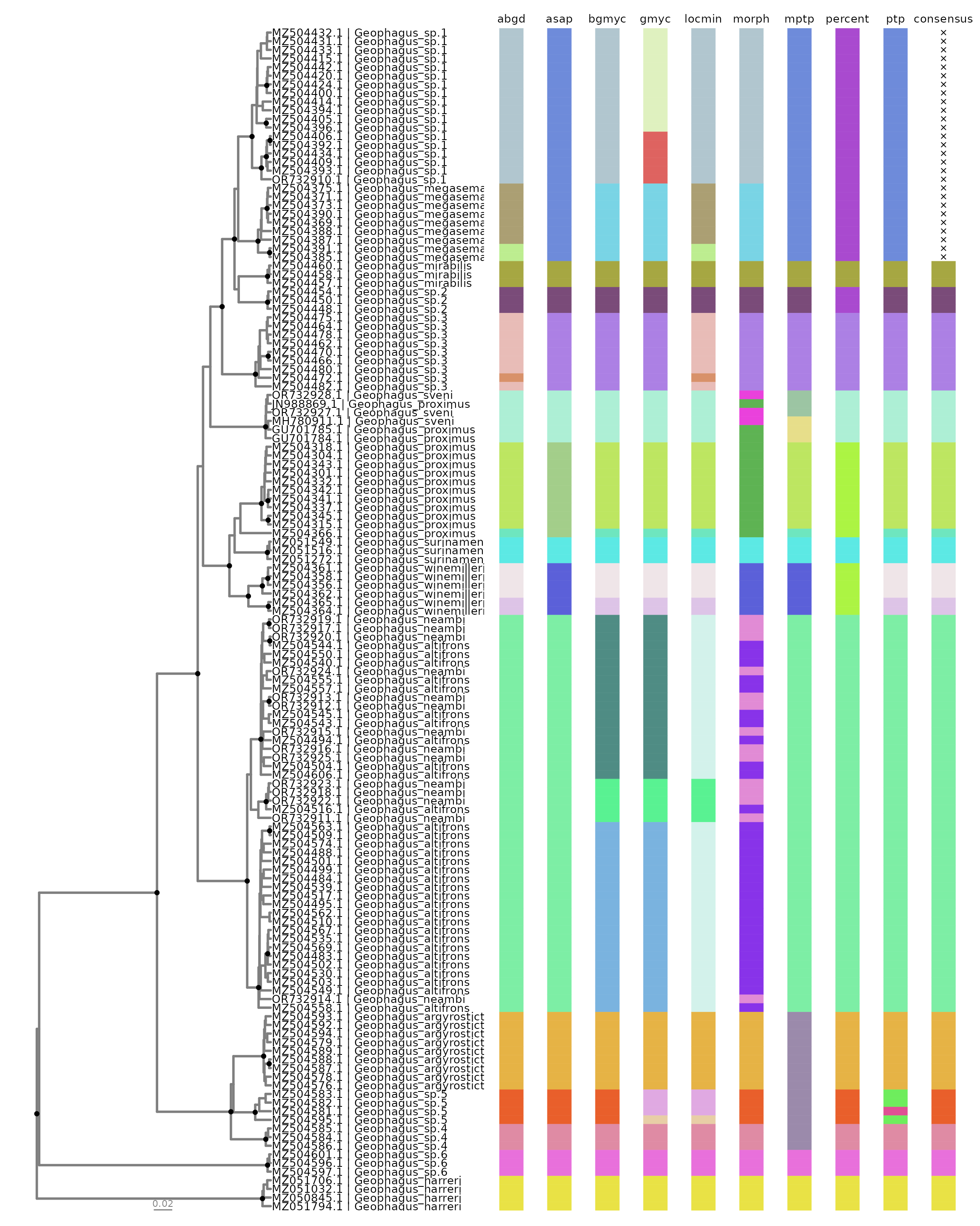
#> # ℹ 127 more rows

Visualizing Results

We can visualize the results by using delim_autoplot. This function will plot a phylogenetic tree alongside with the results contained in all_delims_df. We will use the geophagus_beast tree to visualize the results:


# customize tip labels of the tree
tip_tab <- geophagus_info |> 
  dplyr::filter(gbAccession %in% geophagus_beast@phylo$tip.label) |>
  dplyr::mutate(labs= glue::glue("{gbAccession} | {scientificName}")) |> 
  dplyr::select(gbAccession, labs, scientificName)

# create a customized color palette
cols <- delim_brewer(delim= all_delims_df, package="randomcoloR", seed=42)

# plot
delim_autoplot(all_delims_df, 
               geophagus_beast,
               consensus= TRUE,
               n_match = 5,
               tbl_labs= tip_tab,
               col_vec= cols,
               hexpand= 0.7,
               widths = c(0.5, 0.5))
#> Warning: ⚠ Argument `delim_order` not provided. Using default order from
#> `all_delims_df`.